
In the previous post about high level fixed point arithmetic in vhdl we used a simple elaboration time functions to abstract the bit level manipulations of fixed point number in our filter code code. The ideas were tested with a 6th order Chebyshev type 1 filter that was used to filter a 20MHz sigma delta datastream with Efinix Titanium FPGA. With 32 bit word length used for the filter, the filter implementation used approximately 1000 logic slices as well 37 DSP units.
Due to the way the code was written, we were inferring a separate multiplier for each multiplication needed by the filter with all of the synthesized hardware multipliers used only once with each calculation cycle. Since the DSP slices can perform a new operation every clock cycle and the calculations run every 6 clock cycles, the presented implementation was quite costly in terms of the used dsp slices compared to the amount of calculations the FPGA is capable of. To improve the utilization and reduce the number of these blocks we have the possibility for running multiple operations through a single DSP block.
In this post we will do a walkthrough of taking the second order section module from last post and redesign it such that the implementation shares the DSP elements for the operations in a second order section. The Efinity project along with project sources can be found in the projects repository and the filter module is found on the hVHDL fixed point library.
Filtering with VHDL
The header figure of this post presents the general building block of high order filter, the cascaded second order structure also known as biquad. If we were to write a fully parallel version of the biquad filter, we would get the following algorithm.
y  := b0*u + x1;
x1 <= b1*u - a1*y + x2
x2 <= b2*u - a2*y
What makes this fully parallel filter implementation very expensive, are the 5 multipliers. If they are run at the same time, we need 5 separate hardware multipliers for this algorithm. In the test hardware implementation the filter was operated with a clock of 120MHz and the sigma delta modulator is running at 20 MHz, thus a fully parallel operation is unnecessary since we have 6 clock cycles between each new data bit.
To reduce the number of synthesized hardware multiplers we can use the available 6 clock cycles to mux multiple inputs through a single inferred multiplier in a sequence instead of running each multiplication through separate hardware in parallel. By doing this we exchange specialized and hence costly DSP elements to lower cost registers and muxes. Especially in FPGAs we often run out of logic and DSP elements long before registers are used up, hence this is often a very desirable tradeoff.
We can write a sequential version of the biquad as follows
step 1 : y  <= b0*u + x1;
step 2 : x1 <= b1*u + x2
step 3 : x2 <= b2*u + 0
step 4 : x1 <= (-a1)*y + x1;
step 5 : x2 <= (-a2)*y + x2;
In the algorithm above, we can see that the filter consists of 5 consecutive multiply-add operations. The output y is calculated in step 1 and the result is used in step 4. The calculation of x1 is split into steps 2 and 4 and calculation of x2 is in steps 3 and 5.
Describing reusable hardware with VHDL
This serial version of the filter algorithm has only one multiply-add function active at a time, therefore we can reuse the same multiply-add hardware for all of the operations.
We can create the multiply-add logic just by using the overloaded multiplier operator “*” that was shown in the previous post
  function "*" ( left: integer; right : integer)
        return integer
        is
        begin
            return work.multiplier_pkg.radix_multiply(left,right, word_length, fractional_bits);
        end "*";
With the overloaded “*” operator the multiply-add can be written as
multiply_add_result <= a * b + c;In VHDL describing circuits that reuse hardware resources is quite simple. To use this multiply-add function for multiple separate inputs, we simply assign the signals a, b and c with the gains and signals of the filter and then read the result from multiply_add_result. Using this idea the algorithm can be written as
process(system_clock)
is
    ----
    function "*" ( left: integer; right : integer)
    return integer is
    begin
            return work.multiplier_pkg.radix_multiply(left,right, word_length, fractional_bits);
    end "*";
    ----
begin
    if rising_edge(system_clock) then
        multiply_add_result <= a * b + c;
        CASE program_counter is
            WHEN 0 => a <= u;  b <= b0;  c <= x1; --u*b0 + x1
            WHEN 1 => a <= u;  b <= b1;  c <= x2; --u*b1 + x2
            WHEN 2 => a <= u;  b <= b2;  c <= 0;  --u*b2 + 0
            WHEN 3 => a <= y;  b <= -a1; c <= multiply_add_result;
            WHEN 4 => a <= y;  b <= -a2; c <= multiply_add_result;
            WHEN others => -- do nothing
        end CASE;

        CASE program_counter is
            WHEN 2 => y  <= multiply_add_result;
            WHEN 3 => x1 <= multiply_add_result;
            WHEN 4 => x2 <= multiply_add_result;
            WHEN 5 => x1 <= multiply_add_result;
            WHEN 6 => x2 <= multiply_add_result;
            WHEN others => -- do nothing
        end CASE;
        --
        if program_counter < 6 then
            program_counter <= program_counter + 1;
        else
            program_counter <= 0;
        end if;
        --
    end if;
end process;
Note that I have separated the input and output signal assignments into separate case statements for easier readability. Both use the same program_counter and the values in the two case statements overlap with both having operations defined for 2, 3 and 4. With the separate case statements the logical order of input and output operations is preserved despite the fact that some of them happen simultaneously. In step 2 we are also running the pure multiplication through the same multiply-add function as the signal c assigned to zero.
Subroutine for the multiply-add command
The only issue with the muxing is that it makes the code more difficult to read. To write the VHDL code using the same word “multiply-add” that I have been using to describe the operations that we are invoking, we can make this basic dsp functionality into a callable module. In VHDL this can be done by defining a composite type called record which describes the signals needed by the multiply-add and procedure and functions to create logic and operations from the record signals.
The record holds the input signals a,b and c and the output signal “multiply_add”. The actual functionality is then created with a procedure called create_fixed_point_dsp and the control of this logic that does the signal assignment is done using the multiply and multiply_add procedures and result is obtained with get_dsp_result function.
With these subroutine definitions we separate the different assignments and operations into procedure calls which allows us to give the set of operations descriptive names. The implementations are as follows
------------------------------------------------------------------------
    type fixed_point_dsp_record is record
        a,b,c, multiply_add_output : integer;
    end record;

    constant init_fixed_point_dsp : fixed_point_dsp_record := (0,0,0,0);
------------------------------------------------------------------------
    procedure create_fixed_point_dsp
    (
        signal self : inout fixed_point_dsp_record
    ) is
    begin
        self.multiply_add_output <= self.a * self.b + self.c;

    end create_fixed_point_dsp;
------------------------------------------------------------------------
    function get_dsp_result
    (
        dsp_object : fixed_point_dsp_record
    )
    return integer
    is
    begin
        return dsp_object.multiply_add_output;
    end get_dsp_result;
------------------------------------------------------------------------
    procedure multiply_add
    (
        signal dsp_object : out fixed_point_dsp_record;
        a, b, c : in integer
    ) is
    begin
        dsp_object.a <= a;
        dsp_object.b <= b;
        dsp_object.c <= c;

    end multiply_add;
------------------------------------------------------------------------
    procedure multiply
    (
        signal dsp_object : out fixed_point_dsp_record;
        a, b, c : in integer
    ) is
    begin
        dsp_object.a <= a;
        dsp_object.b <= b;
        dsp_object.c <= 0;

    end multiply_add;
------------------------------------------------------------------------
With these named operations, we can make the code substantially more readable by using the procedures and functions to create the logic instead of the signal assignments directly. With these type and subroutines the exact same filter code from above can be written as
create_fixed_point_dsp(fixed_point_dsp);

if program_counter < 6 then
    program_counter <= program_counter + 1;
end if;
CASE program_counter is
    WHEN 0 => multiply_add(u, b0, x1);
    WHEN 1 => multiply_add(u, b1, x2);
    WHEN 2 => multiply(u, b2);
    WHEN 3 => multiply_add(y, -a1, x1);
    WHEN 4 => multiply_add(y, -a2, x2);
    WHEN others => -- do nothing
end CASE;

CASE program_counter is
    WHEN 2 => y  <= get_dsp_result(fixed_point_dsp);
    WHEN 3 => x1 <= get_dsp_result(fixed_point_dsp);
    WHEN 4 => x2 <= get_dsp_result(fixed_point_dsp);
    WHEN 5 => x1 <= get_dsp_result(fixed_point_dsp);
    WHEN 6 => x2 <= get_dsp_result(fixed_point_dsp);
    WHEN others => -- do nothing
end CASE;
Comparing this implementation to the previous without the record and subroutines, the code is much more descriptive as to what hardware elements it is using and implementation now is given name that describes the behavior of the code instead how it is implemented using muxes.
Biquad filter records and subroutines
What we have created now is a dsp module that can do multiply and multiply-add operations that are then used to create a filter functionality. Continuing with the concept of naming operations, next we can take the filter code and put that into its own record and procedures. The filter module has the record and subroutine description as given below.
------------------------------------------------------------------------
    type sos_filter_record is record
        y, x1, x2, u               : integer;
        state_counter              : integer;
        result_counter             : integer;
        sos_filter_is_ready        : boolean;
        sos_filter_output_is_ready : boolean;
    end record;

    constant init_sos_filter : sos_filter_record := (0,0,0,0,5,5,false,false);
------------------------------------------------------------------------
    procedure create_sos_filter_and_dsp (
        signal self : inout sos_filter_record;
        signal dsp  : inout fixed_point_dsp_record;
        b_gains     : in fix_array;
        a_gains     : in fix_array);

------------------------------------------------------------------------
    procedure request_sos_filter (
        signal sos_filter : out sos_filter_record;
        input_signal : in integer);
------------------------------------------------------------------------
    function get_sos_filter_output ( sos_filter : sos_filter_record)
        return integer;
------------------------------------------------------------------------
The full implementation code can be found here. Note that the implementation is simply the state machine given above now moved into an own procedure with the signals now being defined collectively in the record.
With this sos filter module, the filter implementation can be written in our VHDL code with just 5 lines of VHDL. A pair of signal declarations, a pair of procedure calls and a constant or a signal that holds the gains
-- in architecture
signal fixed_point_dsp : fixed_point_dsp_record := init_fixed_point_dsp;
signal sos_filter1 : sos_filter_record := init_sos_filter;
constant fix_b1 : fix_array(0 to 2) := to_fixed((1.10112824474792e-003  , 2.19578135597009e-003  , 1.09466577037144e-003));
constant fix_a1 : fix_array(0 to 2) := to_fixed((1.00000000000000e+000  , -1.97840025988718e+000 , 987.883963652581e-003));
-- in a clocked process
create_sos_filter_and_dsp(sos_filter, fixed_point_dsp, fix_b1, fix_a1);
Cascading second order sections for higher order filters
Since we use filters with higher order than 2, we commonly want to cascade second order sections. To make this easy we can write a cascade procedure which replaces an if sos1 is ready then trigger sos2 statement with a procedure call called cascade_sos_filters
------------------------------------------------------------------------
    procedure cascade_sos_filters
    (
        signal triggering_sos_filter : inout sos_filter_record;
        signal triggered_sos_filter : inout sos_filter_record
    ) is
    begin
        if sos_filter_out_is_ready(triggering_sos_filter) then
            request_sos_filter(triggered_sos_filter, get_sos_filter_output(triggering_sos_filter));
        end if;
    end cascade_sos_filters;
Finally with this cascade procedure we can create the 6th order fixed point Chebyshev filter from previous post using the sos sections with the following code.
create_sos_filter_and_dsp(sos_filter1, fixed_point_dsp1, fix_b1, fix_a1);
create_sos_filter_and_dsp(sos_filter2, fixed_point_dsp2, fix_b2, fix_a2);
create_sos_filter_and_dsp(sos_filter3, fixed_point_dsp3, fix_b3, fix_a3);

cascade_sos_filters(sos_filter1, sos_filter2);
cascade_sos_filters(sos_filter2, sos_filter3);

if sdm_bit_is_ready then
    request_sos_filter(sos, to_fixed(sdm_bit));
end if;
Note that since the dsp record signal is in the argument list instead of as part of the sos filter record. Because the dsp is defined separately, it is very easy to share the same dsp module over multiple sos filters by just setting the same dsp to multiple create_sos_filter procedures. So if we had more clock cycles for calculations, we could run all of the sos filters through a single dsp if the code was written with all sos filters having the same dsp signal in their argument list
create_sos_filter_and_dsp(sos_filter1, shared_dsp, fix_b1, fix_a1);
create_sos_filter(sos_filter2, shared_dsp, fix_b2, fix_a2);
create_sos_filter(sos_filter3, shared_dsp, fix_b3, fix_a3);

cascade_sos_filters(sos_filter1, sos_filter2);
cascade_sos_filters(sos_filter2, sos_filter3);

if sdm_bit_is_ready then
    request_sos_filter(sos, to_fixed(sdm_bit));
end if;
There is also a testbench which runs the sos filter with real numbers, with the previous implementation and with the shared dsp implementation. The testbench can be launched with the vunit_run script that is found in the repository and the step responce of the three implementations can be seen below

Filtering a delta sigma stream with Efinix Titanium
As we did before, we test the fixed point algorithm with Efinix titanium evaluation kit. The FPGA is connected to Analog Devices ADuM7701 Sigma-Delta ADC evaluation kit and a Digilent Analog Discovery Pro is used as the waveform generator. The sources and the Efinix Efinity project can be found in the projects repository: hVHDL_example_project_with_sigma_delta.

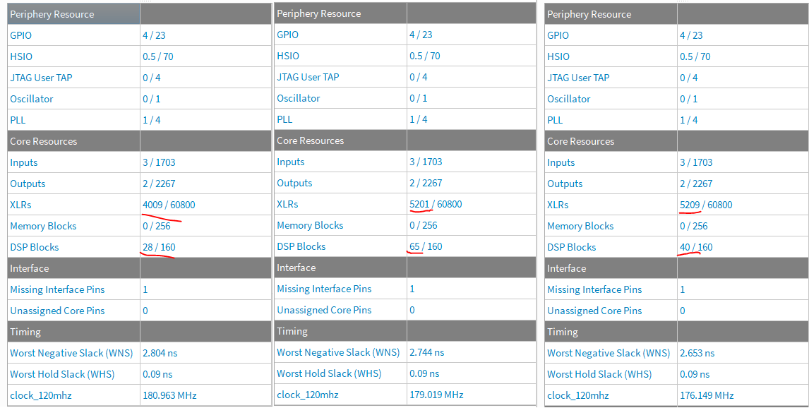
Synthesizing the improved filter module into the Efinix Titanium, we can indeed see that the required resources compared to the design with the filter and without it is only 12 dsp slices instead of 37 and it uses the same amount of around 1000 logic units. This represents space saving of around 70% of the dsp units with no penalty to performance.
First the the ADUM is fed with a sine wave signal and the responces are shown in figure generator is Analog Discovery Pro and it is producing a 90mV peak to peak signal that is read by the adum board and the bit stream is filtered with the fpga and the streamed out from uart to PC.

With the analog discovery pro we can also test various other signal types, like square and triangle waves. With the square wave input, we can see the characteristic overshoot in the chebyshev step responce.


Acknowledgment
I actually won the analog discovery pro in a giveaway, so great big thank you to both electronics-lab.com and Digilent for arranging it! The Analog Discovery pro 3450 has been a fantastic addition to my tools and both the device and the software are very convenient to use.
Notes
We created a second order section filter, but along with it we also branched off a fixed point dsp module which allows us to reuse multiply and add operations also outside of the sos filter. Both of these modules have their individual tests and we can add configurability to the modules further by adding a package that stores the word lengths.
With these modules we managed to lower the DSP resource utilization by a factor of 3 compared to the original implementation with practically no effect on the maximum achievable clock speed. What is interesting here is that the logic resource use was almost identical to the previous implementation which indicates that a sum and a mux use approximately the same amount of logic slices in the Efinix Titanium. We could possibly further lower the logic use by using memory to store the filter gains, since then there would not need to be as many muxes as the gains could come from a single memory port.
The use of abstraction allows code to be written using same words and phrases that describe the problem what it is solving. This is also evident by the fact that despite the code being fixed point, we did not need to consider any fixed point operations specifically here.. The specifics of the fixed point calculation like the scaling by fraction length are actually done under the hood by the to_fixed function calls that were reused as is from the previous blog. This is despite there being a complete rewrite of the the underlying algorithm.