
When we are implementing mathematical algorithms with FPGAs, among the first choices is between a fixed point and floating point arithmetic. As discussed in a post about floating point arithmetic, the use of floats requires the use of variable shift registers which are quite expensive in terms of logic gates. These shifts are not generally needed with fixed point and therefore fixed point is usually substantially less costly to implement. Because there is a speed and area advantage, fixed point is usually the first thing we go for whenever we need to perform math in our FPGA designs.
When we calculate in fixed point, we usually think of integers to save our numbers in the registers of our digital system. Since integers and even hex values are relatively easy to comprehend, more often than not we write these register values directly and keep in our heads what the actual number is that we are representing. This is in contrast to floating point where we use decimal numbers that are converted to from decimal numbers to register values by our compilers and interpreters.
In this post I discuss how to add an abstraction layer to synthesizable fixed point arithmetic which allows us to use real numbers as input values to our code. This substantially simplifies our fixed point code and the abstraction allows us make the algorithms run with configurable word lengths. To test this idea in practice we will design and implement a 6th order low pass chebyshev filter and use it to filter a sigma delta bitstream. Thie filter application is then tested with Efinix Titanium Evaluation kit and a sigma delta adc. All of the referenced sources can be found from the github repository hVHDL_example_project_with_sigma_delta.
Numbers in digital systems
When we read and write numbers we use decimal numbers. These are the common numbers like 7.54 \, , -3.158\, \text{or} \, \pi. Real numbers are what we are most used to look at and thus are most useful when writing calculations. In VHDL we use the datatype ‘real’ to refer to what commonly is thought of when talking about numbers. The real datatype is not synthesizable, but real data types can be used as constants and in functions that are run during elaboration. At the register level, numbers are stored in binary format inside the FPGA.
Both fixed and floating point numbers are stored and used in binary format. Fixed and floating point numbers can be though of as real numbers with some scaling factor that is some desired power of 2. The difference between floating and fixed point is that in floating point the scaling is stored in registers and used dynamically along with the binary number and in fixed point the scaling is coded into the algorithm.
Fixed point numbers
Fixed point numbers are stored in register as bits. N bit register has 2^{\rm N} values it can represent. When the register is interpreted as binary coded integers these register values span the range from 0 to 2^{\rm N} – 1 which for example N=16 bits means numbers from 0 to 65535.
If we take a string of 16 ones in a bit vector
constant maximum_value_in_16_bit : std_logic_vector := "1111_1111_1111_1111";this corresponds to integer which is sum of all integer powers of 2 added together as follows
To represent real numbers with fractional parts like 3.7 in fixed point, we assign some of the bits of the word to integer part or equivalently positive powers of 2 and rest to the fractional part or equivalently negative powers of two. In doing this we can think of choosing the position or fixing the position of the point separating integer and fractional bits. For example if we use 3 bits for the integer part for the 16 bit register of all ones we get
Interpreted like this, the 16 bit fixed point number with 3 integer bits would represent a number range from 0 to ~7.9999. The fractional length here is 13 and it corresponds with the highest negative power of the fractional part which is 2^{-13} in our example.
When we talk about fixed point scaling, what we refer to is this choice of the position of the point in the number.
We can convert any real number to corresponding fixed point register value by multiplying it with a conversion of 2^{fractional \,length}. If we were to convert the real number 3.7 to fixed point with 13 fractional bits we would be storing a register value of 30310 since
In this example, the 3.7\cdot 2^{13} is the fixed point number and the 30310 is the register value interpreted as an integer.
Note that it is very easy to mix the fixed point numbers and corresponding integer values of the registers. To emphasize the difference I will use a notation of number and its fixed point scaling, for example 3.7 \cdot 2^{13} to represent fixed point numbers and integers like 30310 to represent the register values.
Negative numbers
In VHDL negative numbers are encoded with 2’s complement format. The 2’s complement allows add and subtract work with same hardware for both signed or unsigned numbers. Another benefit of 2’s complement is that in a string of additions, overflows in the intermediate parts of the calculation do not matter if the result is in the correct number range.
The way fixed point and integer numbers are encoded in bits using 2’s complement is shown below in a number wheel. Going clockwise, we add 1 to the register value. At the limit, numbers wrap around from positive maximum to negative maximum. Note that the number range of the register is not symmetric between positive and negative numbers as it spans [-2^{word\,length-1}, 2^{word\,length – 1} – 1 ] which corresponds to [-4, 3 ] in 3 bit signed integers and equals [-2.0, 1.5] in fixed point as shown in the figure below.
In most cases we do not need to care much about the encoding of the negative numbers but the 2’s complement is the most used in most of integer arithmetic processors and circuits. Since the conversion between real numbers and fixed point is done using the length of the fractional part it does not directly matter if the number is negative or positive.
Fixed point conversions in VHDL
In order to make fixed point simple to use we will use the real valued numbers as input to functions and have the tools convert these to register values during synthesis. As mentioned, even though the data type real is not synthesizable, there is nothing prevent us from using them as constants to functions that result in synthesizable data types. So even though this is not synthesizable
signal not_synthesizable : real := 4.756;, this is completely valid as the signal data type is integer which is synthesizable
signal completely_synthesizable : integer := integer(3.7*2.0**13.0);The use of completely_synthesizable in rtl results in an integer signal that is instantiated with a value of 30310 which is the result of (3.7*2.0**13) and represents the real value of 3.7 in fixed point correspondingly. Typing the real value in the code is very useful as it tells the reader immediately as to what number we are representing in the code without it needing to be put into a comment. Typing the scaling also shows what fractional length we are using and this information is used by the synthesis.
To make the use of the simple conversion between real values and fixed point even more understandable, we are going to define a function for the conversion.
    function to_fixed
    (
        number : real;
        fractional_bit_length : natural
    )
    return integer
    is
    begin
        return integer(number*2.0**(fractional_bit_length));
    end to_fixed;
For use in testbenches, we also define a function that converts fixed point back to real.
    function to_real
    (
        fixed_point_number : integer;
        number_of_fracional_bits : natural
    )
    return real
    is
    begin
        return real(fixed_point_number)/2.0**fractional_bit_length;
    end to_fixed;
We use the to_fixed to convert number from real values to fixed point and to_real function in our testbenches to convert the register values to human readable real numbers. This also allows us to vary the word lengths to test for algorithm accuracy without changing the testbench. This way the real values act as a layer of abstraction between the numbers that we want to use and the actual register values that are being synthesized in the hardware.
signal example : integer := to_fixed(number => 3.7, fractional_bit_length => 13);Since VHDL allows overloading, we can make this even simpler by locally defining an overloaded to_fixed function with constant fractional length
    function to_fixed
    (
        number : real;
    )
    return integer
    is
        constant fractional_bit_length : natural := 13;
    begin
        return to_fixed(number, fractional_bit_length);
    end to_fixed;
This makes the fixed point numbers even more readable in the source code
signal example : integer := to_fixed(3.7);
signal another_example : integer := to_fixed(-2.2);
We can define this overload in any of the declarative regions in VHDL where functions can be declared, which includes bodies of packages and the region between words “is” and “begin” in functions, procedures, processes and architectures.
Fixed point word length
When we design with VHDL we are actually designing customized hardware. This means that we are not bound to calculating in any specific word lengths. Because of this we can choose any number of bits that fit the precision and dynamic range needed in our calculations.
There are two ways to increase the word length. We can either increase the number of integer bits or the length of the fractional part. This is illustrated in Figure 2.

In practical terms the number range, which determines the number of integer bits that we need, is determined by the algorithm that we are implementing. Hence with VHDL the word length is mostly used to tune our accuracy by trimming the fractional part and the number of integer bits is constant and defined by the algorithm that we are implementing. The way we fix the integer bit width is simply by defining constants for word length and integer bits and use them to calculate the number of fractional bits.
    constant word_length  : integer := 32;
    constant integer_bits : integer := 8;
    constant fractional_bits : integer := word_length-integer_bits;
Fixed point arithmetic in VHDL
Doing arithmetic in fixed point is quite straightforward. For additions and subtractions we can just use the “+” and “-” operators as is given that we have consistent fractional length during our calculation. We can mix and match dissimilar word lengths as long as the fractional parts have equal length. We also need to know that the result fits in the result register.
For example, adding numbers 3 and 1 in fixed point with equal fractional parts corresponds with the following operation
With the fixed point conversion functions this can be written in VHDL as follows
a := to_fixed(fixed_point_number => 3.0, number_of_fracional_bits => 3);
b := to_fixed(fixed_point_number => 1.0, number_of_fracional_bits => 3);

result <= a + b;
In direct register values this corresponds to adding together integers
If the fractional lengths were not equal, then we would either left or right shift one of the words to scale the number into the same range.
Multiplication
Multiplication with fixed point works in two parts. We first multiply the numbers together and then the result is shifted to desired fixed point value.
Let’s consider multiplying the same numbers together using the radix_multiply function with arbitrarily assigning 13 and 6 to the fractional lengths. This yields the following
From the result 3.0(2^{13}\cdot 2^6) we can see that the result has a fractional length that is the sum of the bit widths of the multiplied numbers. The result can be returned to original scale read by dividing the result with the fixed point scaling of the multiplicant2^6. In binary this is equivalent to right shifting by 6. Multiplication thus works between fixed point numbers with any fractional bit widths as long as we know what the fixed point scaling of the multiplicant is.
The function to do fixed point multiplication has 3 arguments. It needs to know the word length which can be read from the length of the input and it needs t know the number of fractional bits of the multiplicand to return the correct result. The word “radix” in the function refers to the placement of the point in the number that corresponds with the final shifting of the result. The bit slicing of the return value is just another way to write a right shift.
    function radix_multiply
    (
        left, right : signed;
        radix       : natural
    )
    return signed
    is
        constant word_length : natural := left'length + right'length;
        variable result : signed(word_length-1 downto 0);
    begin
        result := left * right;
        return result(left'length+radix-1 downto radix);
    end radix_multiply;
With the radix multiply, the fixed point multiplication can be invoked with a function call
result <= radix_multiply(to_fixed(3.0, 13), to_fixed(1.0, 6), 6);VHDL allows overloading of operators, hence we can use the radix multiply to define the “*” operator to work directly with integers.
        function "*" ( left: integer; right : integer)
        return integer
        is
        begin
            return work.multiplier_pkg.radix_multiply(left,right, word_length, 6);
        end "*";
, with this overload we can use the * directly between numbers to perform a fixed point multiplication as seen in the snippet below
result <= to_fixed(3.0, 13) * to_fixed(1.0, 6);Note that this method for doing a multiplication is not pipelined and requires a separate multiplier to be synthesized for each multiplication. For a pipelined version of a multiplier, see the multiplier module and its test bench in the hVHDL fixed point library.
Filter implementation using Fixed point
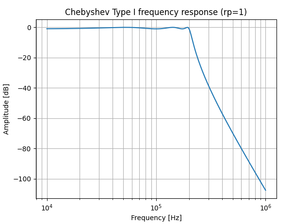
To show how to use fixed point arithmetic, we will create a low pass filter for sigma delta filter. The synthesizable filter package can be found in the hVHDL fixed point repository and the testbench is found here. For filtering we are going to use a 6th order Chebyshev type filter. The filter is calculated at the bit frequency of the sigma delta modulator, hence we will choose the bandwidth based on the desired signal to noise ratio of the sigma delta modulated bit stream. In this case we will choose bandwidth of 1/30.
The matlab script to get the filter gains is shown below. I would prefer to use python and scipy library for the filter design, but currently I do not know how to get the comparable gains using Python, hence matlab was used.
% matlab script for generating the gains of a
% chebyshev type 1 filter with 1/30 bandwidth
[b,a] = cheby1(6, 1, 1/30);
[sos, g] = tf2sos(b,a, 'down',2)
Since we have defined functions that translate real values to fixed point, we can write the gains directly to the VHDL source as given by the matlab algorithm.
    constant fix_b1 : fix_array(0 to 2) := to_fixed((1.10112824474792e-003  , 2.19578135597009e-003  , 1.09466577037144e-003));
    constant fix_b2 : fix_array(0 to 2) := to_fixed((1.16088276025753e-003  , 2.32172985621810e-003  , 1.16086054728631e-003));
    constant fix_b3 : fix_array(0 to 2) := to_fixed(((42.4644359704529e-003 , 85.1798866651586e-003  , 42.7159465798333e-003) / 58.875768));

    constant fix_a1 : fix_array(0 to 2) := to_fixed((1.00000000000000e+000  , -1.97840025988718e+000 , 987.883963652581e-003));
    constant fix_a2 : fix_array(0 to 2) := to_fixed((1.00000000000000e+000  , -1.96191974906017e+000 , 967.208461633959e-003));
    constant fix_a3 : fix_array(0 to 2) := to_fixed((1.00000000000000e+000  , -1.95425095615658e+000 , 955.427665692536e-003));
The frequency responce in Figure 3 shows classic Chebyshev filter responce with ripple in the passband and fast transition to stop band.
The testbench implements a fixed point and a real valued version of the filter and compares the outputs. The step responces are of the two implementations are show in Figure 4 below. Filter_out signals are the second order section outputs of the real valued implementation and fix_filter out shows the fixed point filter outputs. Note that the fixed point filters show the raw integer values of the registers.

The filter is implemented using a cascaded second order filter structure also known as biquads whose structure is shown in Figure 5 below. The reason for using cascaded second order section structure is that it has good stability and has good round-off noise characteristics and it is the recommended structure in the in python scipy library. The a and b refer to the filter gains and x1 and x2 refer to the filter memory values.

The corresponding filter is implemented in a procedure that takes in the gains, input and output signals, a counter and produces an output of the filtered result. The multiplier is overloaded using the radix_multiply function in the procedure to allow for using just the “*” operator inside the procedure.
------------------------------------------------------------------------
    procedure calculate_sos
    (
        signal memory : inout fix_array;
        input         : in integer;
        signal output : inout integer;
        counter       : in integer;
        b_gains       : in fix_array;
        a_gains       : in fix_array;
        constant counter_offset : in integer
    ) is
    --------------------------
        function "*" ( left: integer; right : integer)
        return integer
        is
        begin
            return work.multiplier_pkg.radix_multiply(left,right, word_length, fractional_bits);
        end "*";
    --------------------------
    begin
        if counter = 0 + counter_offset then output    <= input * b_gains(0) + memory(0);                       end if;
        if counter = 1 + counter_offset then memory(0) <= input * b_gains(1) - output * a_gains(1) + memory(1); end if;
        if counter = 2 + counter_offset then memory(1) <= input * b_gains(2) - output * a_gains(2);             end if;

    end calculate_sos;
The calculation sequence is implemented using if statements, as this allows adding an offset to the counter that sequences the calculations. The first sos section is calculated with counter values 0, 1 and 2, the second sos section is started one clock cycle later and spans the clocks 1,2,3 and the third section is started with 2 clock cycles later and is calculated with cycles 2,3,4. This is illustrated in below

The use of the counter offset allows the 3 sections to be implemented in 3 procedure calls with the last number in the call being the counter offset at which point the calculations are started
            if state_counter < 5 then
                state_counter <= state_counter + 1;
            end if;
            calculate_sos(fix_memory1 , to_fixed(cic_filter_data) , fix_filter_out  , state_counter , fix_b1 , fix_a1 , 0);
            calculate_sos(fix_memory2 , fix_filter_out            , fix_filter_out1 , state_counter , fix_b2 , fix_a2 , 1);
            calculate_sos(fix_memory3 , fix_filter_out1           , fix_filter_out2 , state_counter , fix_b3 , fix_a3 , 2);
The filter is started by setting the counter to zero at the time when the filter is to be started.
if sdm_clock_counter = sample_instant then
    state_counter <= 0;
end if;
The entity with the full filter implementation can be found here. Note that the entity has 3 different filters and the connection to the internal bus that is accessible by UART.
Filtering a delta sigma stream with Efinix Titanium
We test the fixed point algorithm with Efinix titanium evaluation kit. This is very convenient kit to use since it has onboard uart that connects to the same usb cable as the jtag. The FPGA is connected to Analog Devices ADuM7701 Sigma-Delta ADC evaluation kit. ADuM7701 is a sigma-delta modulator, which means that we input a clock and the modulator sends out a bit stream that represents the analog voltage. The sigma-delta is read by filtering the 1 bit stream with the Chebyshev filter at the bit clock, that is run at 20MHz. The only connections between the boards are the 3.3V IO and ground as well as the data and clock signals to read the sigma delta bit stream. The sources can be found in the projects repository: hVHDL_example_project_with_sigma_delta.

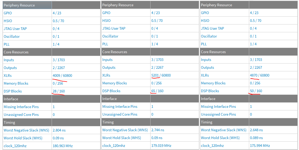
The resource usage of the filter is illustrated below. Since the project has additional features, the resource use is shown without the IIR filter, with 32 bit word length and with 26 bit word length. The 32 bit word length requires 1200 logic units and 37 dsp cores which reduces to 900 logic and 22 dsp units with 26 bit word length.
Because of the used abstraction of the word length, we can change word length of the algorithm by just changing a single constant that is found in the package.
The testbench checks for error more than 1% between the fixed and real valued implementations and it works down to 24 bit word length using the implementation.
The most common method to filter a sigma delta bit stream is to use a cascaded integrator chain (CIC) filter. CIC filter is simply a series of integrators followed by equal number of differentiators that are calculated at every 32th integrator calculation cycle. The project uses this method as the reference in addition to the chebyshev filter. The used VHDL implementation of the CIC filter can be found here.
First the the ADUM is fed with a sine wave signal and the responces are shown in figure generator is Analog Discovery Pro and it is producing a 200mV peak to peak signal that is read by the adum board and the bit stream is filtered with the fpga and the streamed out from uart to PC.

With the analog discovery pro we can also test various other signal types, like square and triangle waves. With the square wave input, we can see the characteristic overshoot in the chebyshev step responce.


Final notes
The implementation discussed here uses comparatively lots of dsp resources. This is because all multiplications use their own multiplier. With increasing word lengths we would want to pipeline the operations and also try to reuse the multipliers to save up on the resource use. The FPGA implementation also has a bank of four cascaded first order filters that can be implemented without any dsp cores given that the filter gain corresponds with a bit shift.
VHDL2008 standard has fixed point package that has types for signed and unsigned fixed point numbers. It also has conversion functions between real and fixed point as well as fixed point and signed/unsigned. The VHDL2008 fixed point package also has functions for rounding. The procedures shown in this post functions could be written using the fixed point library, however free version of intel Quartus does not currently support VHDL2008 and I have lots of hardware that uses intel FPGAs.