An electric motor is a device that is used to produce 90% of electricity and what consumes approximately half of it globally. Electrical motors allows the control of motion through production of torque by controlling the currents in the motors windings. Motors are controlled with a device called inverter, or equivalently a variable frequency converter which controls the currents of the motor by changing the motor voltage.

For a great primer on motor windings and their torque production see this video Understanding electric motor Windings! and for how a motor is controlled see this video Tesla Model 3’s motor. If you are not into Teslas, try to ignore the car as the important part is about magnetic fields and their angles. Also, see here stock Tesla Plaid vs 1000hp McLaren on a drag race.

So this time we design and implement a feedback control system for a model of an internal permanent magnet electrical motor. First we model the motor with differential equations, then we design a control structure based on that model. Lastly the model and the control are implemented in VHDL and used in a real-time simulator running in a Cyclone 10 lp FPGA. The project with all of the sources is found on the projects github repository. The project is developed with libraries in git submodules for easier reuse.

Modeling and control of a Permanent Magnet Electric Motor

The formal mathematical notation regarding electrical motors is extremely dense, but here we are looking at motors from a control engineers point of view. Basically anything with a “ $(t)$ ” is a signal that changes in time and is modeled with differential equations, and all others are arbitrary gains that are somehow affecting the result after we hack ‘n slash (or “tune”) the controller gains for the model. A more explicit explanation on the motor modeling can be found here. See the link to the pdf for Dynamic Model of PM Synchronous Motors by Dal Y. Ohm.

Motor mechanical model

The mechanical model of a motor models the position of the rotating part of motor called rotor. When the rotor is affected with torque, angular acceleration is produced. The amount of acceleration that a torque produces is determined by the inertial mass of the object (J).

As acceleration is a measure of how fast angular speed changes when time passes the speed starts to increase. With non zero speed the angle changes. When translated into mathematics, torque causes acceleration, that integrates into speed that integrates into angle. Using the permanent magnet torque and reluctance torque as the torque inputs this

\begin{align} \dot{\omega}_m(t) &=\frac{1}{\rm J} \bigg[ {\rm T}_{\rm pm} + {\rm T}_{\rm reluctance} \bigg] \\ \dot{\phi}_m &= \omega_m(t) \end{align}

, where J is the moment of inertia. This set of equations models the rotation of the physical rotor as change in angle $\phi(t)_m$ and speed $\omega_m(t)$ .

In electric motors motors there are two main ways that torque is produced. First is direct interaction between current and magnetic field called the Lorenz force. The other is called reluctance force, which is the force that sticks permanent magnets to iron. In synchronous permanent magnet motors, both forms of forces can be utilized in torque production and the resulting torque is the sum of these forces.

Torque in electrical motors

When we consider electric motors we commonly divide current into its components that are aligned with the field $i_d(t)$ or perpendicular to it $i_q(t)$ as shown in Figure 1. The orientations are referred to as direct $(d)$ or quadratic $(q)$ and marked in the subscript.

Lorenz torque

For Lorenz force, the quadratic current $i_q(t)$ is the one that produces the permanent magnet torque ${\rm T_{pm}}$ as the product of the permanent magnet field strength $\psi_{pm}$ and current $i_q(t)$ . The $\psi_{pm}$ is considered to be a constant magnetic of the permanent magnet.

\begin{equation} {\rm T}_{\rm pm} = \psi_{\rm pm}i_q(t) \end{equation}

Reluctance torque

Reluctance is a measure of how well magnetic field is being conducted in a material. When the rotor is constructed in a way that there is air in the construction, drawn in Figure 2 as “+” shaped, then the orientation of the rotor has a high reluctance and low reluctance orientation. The reluctance force is what tries to orient the rotor in a position where where the metal tang is closest to the magnet. If we just rotated a magnet around a similarly shaped metal object it would quite obviously try to follow the magnet

In a motor, the two positions also correspond with the motor inductance, which is a measure on how well electric current produces magnetic field. When the rotor is in the high reluctance orientation, the magnetic field has minimal amount of air that it needs to travel through thus it also produces high field strength with current and it has maximum inductance. In the low reluctance position there is more air, thus lower reluctance and therefore less field is produced with unit of current.

In a motor the magnetic field is produced by the currents in the motor windings. As the rotor rotates synchronously with the field, the two positions also correspond to the d and q direction currents. Thus the two directions also have differing inductances. When the inductance is considered the torque produced by the reluctance force is the difference of the two motor inductances multiplied by both of the d and q currents.

\begin{equation} {\rm T}_{\rm reluctance} = (L_d - L_q)i_d(t)i_q(t) \end{equation}

Motor mechanical model

The magnetic field inside the motor rotates at speed that is relative to the mechanical speed by the number of pole pairs inside the motor. As we actually control the current aligned with the magnetic field inside the motor, we need to model the electrical angle. There is a simple relation between the mechanical and electrical angles on permanent magnet motors that depends on the pole pairs in the motor winding construction

\begin{align} \dot{\omega}_e(t) &= {\rm p}\frac{3}{2}\dot{\omega}_m(t) \\ \dot{\phi}_e &= \omega_e(t) \end{align}

With the pole pairs added to (3) and (4) we get the mechanical model of the motor that produces the electrical angle with the forces caused by the motor currents

\begin{align} \dot{\omega}_e(t) &= {\rm p} \frac{3}{2} \frac{1} {\rm J} \bigg[ \psi_{pm}i_q(t) + (L_d - L_q)i_d(t)i_q(t) - {\rm T}_{\rm L} \bigg] \\ \dot{\phi}_e &= \omega_e(t) \end{align}

The important notion in the equations (7) and (8) is that torque of the motor is determined by the $i_d(t)$ and $i_q(t)$ currents. The currents are caused by the inductances of the motor and the voltage of the inverter.

Motor electrical model

The torque equations are presented in vector form where the current is divided into the field oriented $i_d(t)$ part and the perpendicular $i_q(t)$ part. This separation is also mirrored in the electrical circuit which is divided into direct and quadrature parts.

The d – direction circuit has voltage over the inductance the difference between the back-emf voltage, input voltage and the voltage over the winding resistance. The back emf voltage is what models the voltage caused by magnetic flux and the rotational speed of the magnetic field. The flux is the product of current and inductance thus for d-direction it is modeled by $L_q \cdot \omega_e(t) \cdot i_q(t)$

For the q direction the current model is the the same as in d-direction, but there is also a permanent magnet flux induced voltage that depends on the rotational speed $\omega_e(t)$ . The difference between d and q directions are highlighted.

The electrical model equations that correspond to these circuits for the permanent magnet motor is shown in equations (9) and (10) .

\begin{align} \dot{i}_d(t) &= \frac{1}{\rm L_d}\bigg [-{\rm R}i_d(t) - {\rm L_q}\omega_e(t)i_q(t) + v_d(t) \bigg] \\ \dot{i}_q(t) &= \frac{1}{\rm L_q} \bigg[ { - \rm L_d}\omega_e(t)i_d(t) - {\rm R}i_q(t) - \psi_{pm}\omega_e(t) + v_q(t) \bigg] \end{align}

We obtain the the final motor model as the combination (7) – (10). Thus the permanent magnet motor is described by the following four equations.

\color{#79FE0C} \begin{align} \dot{i}_d(t) &= \frac{1}{\rm L_d}\bigg [-{\rm R}i_d(t) - {\rm L_q}\omega_e(t)i_q(t) + v_d(t) \bigg] \\ \dot{i}_q(t) &= \frac{1}{\rm L_q} \bigg[ { - \rm L_d}\omega_e(t)i_d(t) - {\rm R}i_q(t) - \psi_{pm}\omega_e(t) + v_q(t) \bigg] \\ \dot{\omega}_e(t) &= {\rm p} \frac{3}{2} \frac{1} {\rm J} \bigg[ \psi_{pm}i_q(t) + (L_d - L_q)i_d(t)i_q(t) - {\rm T}_{\rm L} \bigg] \\ \dot{\phi}_e(t) &= \omega_e(t) \end{align}

Where $\psi_{pm}$ is the flux of the permanent magnet $\omega_{e}$ is the angular speed of the magnetic field which is the rotor speed multiplier by the number of pole pairs p. The field angle of the motor is $\phi(t)$ . The controllable input are the voltages $v_d(t)$ and $v_q(t)$ .

The interesting part here is that the two currents are interconnected with the current $i_d(t)$ producing voltage for $i_q(t)$ and $i_q(t)$ producing voltage for the $i_d(t)$ equation. The model is also nonlinear as there are products of the state variables in the equations.

It is this model of the permanent magnet motor that we design the feedback control for. Since the controlled current $i_d(t)$ and $i_q(t)$ are direct and perpendicular relative to the magnetic field inside the rotor, this is called field oriented control.

Field Oriented Current Control

The controlled variables in the motor are the two voltages that are supplied by the inverter $v_d(t)$ and $v_q(t)$ . When we model the feedback operation, we simply replace the controlled voltages $v_d(t)$ and $v_q(t)$ with any desired function of the differential signals in the model.

Since we measure both currents $i_q(t)$ and $i_d(t)$ and the angular speed $\omega(t)$ , we can simply add these terms to the input variable $v_q(t)$ that is controlled to negate their effects in the model. As the system is of first order, we define a PI controller for the $v_d(t)$ as

\begin{align} v_d(t) &= {\rm R}i_d(t) + {\rm L_q}\omega_e(t)i_q(t) - k_{pd}\bigg[i_{d_{ref}}(t) - i_d(t)\bigg] \\&\phantom{=} - k_{id}x_1(t) \\[0.4em] \dot{x}_1(t) &= i_{d_{ref}}(t) - i_d(t) \end{align}

, where $x(t)$ is the integrator state and $[i_{d_{ref}}(t) – i_d(t)]$ is the error term. If we substitute (15)-(17) to (11) we get the feedback controlled state space equation for the $\dot{i}_d(t)$ current as

\begin{align} \dot{i}_d(t) &= \frac{1}{\rm L_d}\bigg (-k_{pd}\bigg[i_{d_{ref}}(t) - i_d(t)\bigg] - k_{id}x_1(t) \bigg ) \\[0.8em] \dot{x}_1(t) &= i_{d_{ref}}(t) - i_d(t) \end{align}

The terms $k_{pd}, k_{id}$ are the tuning parameters for the PI controller, commonly known as the proportional and integral gains.

The $i_q(t)$ controller can be similarly obtained by collecting terms from (12) and adding the pi control gains. The $i_q(t)$ controller is

\begin{align} v_q(t) &= { \rm L_d}\omega_e(t)i_d(t) + {\rm R}i_q(t) - k_{pq}\bigg[i_{q_{ref}}(t) - i_q(t)\bigg] \\ &\phantom{=} -k_{iq}x_2(t) + \psi_{pm}\omega_e(t) \\[0.4em] \dot{x}_2(t) &= \bigg[i_{q_{ref}}(t) - i_q(t)\bigg] \end{align}

The final current controller is thus obtained by collecting together (17) – (21)

\color{#d4af37} \begin{align} v_d(t) &= {\rm R}i_d(t) + {\rm L_q}\omega_e(t)i_q(t) - k_{pd}\bigg[i_{d_{ref}}(t) - i_d(t)\bigg] -k_{id}x_1(t) \\ \dot{x}_1(t) &= \bigg[i_{d_{ref}}(t) - i_d(t)\bigg] \\[0.3em] v_q(t) &= { \rm L_d}\omega_e(t)i_d(t) + {\rm R}i_q(t) - k_{pq}\bigg[i_{q_{ref}}(t) - i_q(t)\bigg] -k_{iq}x_2(t) \\ &\phantom{=} + \psi_{pm}\omega_e(t) \\[0.1em] \dot{x}_2(t) &= \bigg[i_{q_{ref}}(t) - i_q(t)\bigg] \end{align}

Since the control gains can be tuned at will, we can literally assign any arbitrary dynamics to the currents and the final control law that is programmed just a standard PI controller with the additional feed forward terms.

Speed control

The speed of the motor is controlled with the motor torque as given by (1) – (2). The torque equations are interconnected as the reluctance torque is effected by both $i_d(t)$ and $i_q(t)$ . For the sake of simplicity we will run the motor with $i_d(t) = 0$ which removes the reluctance torques effect from the motor. Thus the motor speed is controlled with just the $i_{q_{ref}}(t)$ .

\begin{align} \dot{\omega}_e(t) &= {\rm p} \frac{3}{2} \frac{1} {\rm J} \bigg[ \psi_{pm}i_{q_{ref}}(t) \bigg] \end{align}

The $i_{q_{ref}}(t)$ is calculated with a PI controller where the input is the difference of the speed reference and the measured speed $\omega _{e_{ref}}(t) – \omega _{e}(t)$ .

\color{#d4af37} \begin{align} i_{q_{ref}}(t) &= k_{p{\omega}} \bigg[\omega _{e_{ref}}(t) - \omega _{e}(t)\bigg] + k_{i\omega}x_3(t) \\[0.4em] \dot{x}_3(t) &= \bigg[\omega _{e_{ref}}(t) - \omega _{e}(t)\bigg] \end{align}

We now have all of the parts required for a current control of an electric drive. So next we code the motor model (11) – (14), the current controller (23)-(27) and speed controller (29)-(30) in high level synthesizable VHDL which is then tested with FPGA.

VHDL implementation of motor model and control

The complete motor model is built in a record. The record has members for mechanical model, an electrical model and the electrical angle. These are record types that with their create procedures implement the calculation for the corresponding differential equations. The create_pmsm procedure calls the create procedures for the mechanical and electrical models as well as the electrical angle calculation.

library ieee;
    use ieee.std_logic_1164.all;
    use ieee.numeric_std.all;

library math_library;
    use math_library.multiplier_pkg.all;
    use math_library.state_variable_pkg.all;
    use math_library.pmsm_electrical_model_pkg.all;
    use math_library.pmsm_mechanical_model_pkg.all;

package permanent_magnet_motor_model_pkg is

------------------------------------------------------------------------

    type permanent_magnet_motor_model_record is record
        id_current_model    : id_current_model_record ;
        iq_current_model    : id_current_model_record ;
        angular_speed_model : angular_speed_record    ;
        electrical_angle    : state_variable_record   ;
        vd_input_voltage    : int18                   ;
        vq_input_voltage    : int18                   ;
    end record                                        ;

    constant init_permanent_magnet_motor_model : permanent_magnet_motor_model_record := 
        (init_id_current_model          ,
         init_id_current_model          ,
         init_angular_speed_model       ,
         init_state_variable_gain(3000) ,
         0, 0);

end package permanent_magnet_motor_model_pkg;
------------------------------------------------------------------------
package body permanent_magnet_motor_model_pkg is
    procedure create_pmsm_model
    (
        signal pmsm_model_object : inout permanent_magnet_motor_model_record ;

        signal id_multiplier    : inout multiplier_record ;
        signal iq_multiplier    : inout multiplier_record ;
        signal w_multiplier     : inout multiplier_record ;
        signal angle_multiplier : inout multiplier_record;
        motor_parameters        : in motor_parameter_record
    ) is
 
    begin
        
        --------------------------------------------------
        create_pmsm_electrical_model(
            id_current_model                        ,
            iq_current_model                        ,
            id_multiplier                           ,
            iq_multiplier                           ,
            angular_speed_model.angular_speed.state ,
            vd_input_voltage                        ,
            vq_input_voltage                        ,
            permanent_magnet_flux                   ,
            Ld                                      ,
            Lq                                      ,
            rotor_resistance);

        --------------------------------------------------
        create_angular_speed_model(
            angular_speed_model               ,
            w_multiplier                      ,
            Ld                                ,
            Lq                                ,
            id_current_model.id_current.state ,
            iq_current_model.id_current.state ,
            permanent_magnet_flux);
        --------------------------------------------------
        create_state_variable(electrical_angle,angle_multiplier, to_signed(get_angular_speed(angular_speed_model),18));

    end create_pmsm_model;

Mechanical model

As we have already developed the state-variable datatype previously, we can use that for the state variables in the motor model. For the mechanical model, the state variable is the angular speed.

The angular speed object is built using a record which holds all of the reqisters needed for the calculation. The record has a state variable for the angular speed, a counter for the state machine that performs the calculations.


library math_library;
    use math_library.multiplier_pkg.all;
    use math_library.state_variable_pkg.all;

package pmsm_mechanical_model_pkg is

------------------------------------------------------------------------
    type angular_speed_record is record
        angular_speed                     : state_variable_record;
        angular_speed_calculation_counter : natural range 0 to 15;
        load_torque                       : int18                ;
        w_state_equation                  : int18                ;
        permanent_magnet_torque           : int18                ;
        reluctance_torque                 : int18                ;
        friction                          : int18                ;
    end record;

end package pmsm_mechanical_model_pkg;

The registers are used in a create_angular_speed_model procedure, that has all of the calculations required. The procedure includes the required multiplier object in its interface as this allows sharing the multiplier with for example other parts of the motor model. The motor electrical parameters are also given to the procedure as arguments. This allows changing the parameters without it affecting the model calculation.

The multiplications are pipelined to allow for minimal latency for the calculations.

------------------------------------------------------------------------
    procedure create_angular_speed_model
    (
        signal angular_speed_object : inout angular_speed_record;
        signal w_multiplier         : inout multiplier_record;
        Ld                          : int18;
        Lq                          : int18;
        id_current                  : int18;
        iq_current                  : int18;
        permanent_magnet_flux       : int18
    ) is
        alias angular_speed                     is angular_speed_object.angular_speed                     ;
        alias angular_speed_calculation_counter is angular_speed_object.angular_speed_calculation_counter ;
        alias load_torque                       is angular_speed_object.load_torque                       ;
        alias w_state_equation                  is angular_speed_object.w_state_equation                  ;
        alias permanent_magnet_torque           is angular_speed_object.permanent_magnet_torque           ;
        alias reluctance_torque                 is angular_speed_object.reluctance_torque                 ;
        alias friction                          is angular_speed_object.friction                          ;
    begin
        create_state_variable(angular_speed , w_multiplier  , w_state_equation);

        CASE angular_speed_calculation_counter is
            WHEN 0 =>
                multiply(w_multiplier, id_current, iq_current);
                increment(angular_speed_calculation_counter);
            WHEN 1 =>
                multiply(w_multiplier, permanent_magnet_flux, iq_current);
                increment(angular_speed_calculation_counter);
            WHEN 2 =>
                if multiplier_is_ready(w_multiplier) then
                    multiply(w_multiplier, (Ld-Lq), get_multiplier_result(w_multiplier, 15));
                    increment(angular_speed_calculation_counter);
                end if;
            WHEN 3 =>
                multiply(w_multiplier, angular_speed.state, 10e2);
                permanent_magnet_torque <= get_multiplier_result(w_multiplier, 15);
                w_state_equation        <= get_multiplier_result(w_multiplier, 15) - load_torque;
                increment(angular_speed_calculation_counter);
            WHEN 4 =>
                if multiplier_is_ready(w_multiplier) then
                    reluctance_torque <= get_multiplier_result(w_multiplier, 15);
                    w_state_equation <= w_state_equation + get_multiplier_result(w_multiplier, 15);
                    increment(angular_speed_calculation_counter);
                end if;
            WHEN 5 =>
                friction <= - get_multiplier_result(w_multiplier, 15);
                w_state_equation <= w_state_equation - get_multiplier_result(w_multiplier, 15);
                increment(angular_speed_calculation_counter);
            WHEN 6 =>
                request_state_variable_calculation(angular_speed);
                increment(angular_speed_calculation_counter);
            WHEN others =>
        end CASE;
        
    end create_angular_speed_model;

------------------------------------------------------------------------
end package body pmsm_mechanical_model_pkg;

Electrical model

The electrical model is built as a record type that has state variables for the id and iq currents, the model calculation counter and calculation is ready variables. The motor current type is used as we wish to have option for either using a single multiplier and calculating the entire motor model with one DSP slice, or run the calculations in parallel with two DSP slices.

The model calculation is started by setting the id_calculation_counter to zero with the request_calculation procedure. In order to speed up the calculations, the multiplications of the model are pipelined. Since we are calculating linear terms terms we can request both multiplications and then use a register to catch the result once the multiplication is done.

------------------------------------------------------------------------
    procedure create_pmsm_electrical_model
    (
        signal id_current_object : inout id_current_model_record;
        signal iq_current_object : inout id_current_model_record;
        signal id_multiplier     : inout multiplier_record;
        signal iq_multiplier     : inout multiplier_record;
        angular_speed            : in int18;
        vd_input_voltage         : in int18;
        vq_input_voltage         : in int18;
        permanent_magnet_flux    : in int18;
        Ld                       : in int18;
        Lq                       : in int18;
        rotor_resistance         : in int18
    ) is
        alias id_calculation_counter is id_current_object.id_calculation_counter;
        alias id_state_equation      is id_current_object.id_state_equation     ;
        alias id_current             is id_current_object.id_current            ;

        alias iq_calculation_counter is iq_current_object.id_calculation_counter;
        alias iq_state_equation      is iq_current_object.id_state_equation;
        alias iq_current             is iq_current_object.id_current;

    begin
            create_state_variable(id_current    , id_multiplier , id_state_equation);
            create_state_variable(iq_current    , iq_multiplier , iq_state_equation);
            CASE id_calculation_counter is
                -- calculate id state equation
                WHEN 0 =>
                    multiply(id_multiplier, rotor_resistance, id_current.state);
                    increment(id_calculation_counter);
                WHEN 1 =>
                    multiply(id_multiplier, angular_speed, iq_current.state);
                    increment(id_calculation_counter);
                WHEN 2 =>
                    if multiplier_is_ready(id_multiplier) then
                        id_state_equation <= -get_multiplier_result(id_multiplier,15);
                        increment(id_calculation_counter);
                    end if;
                WHEN 3 =>
                    multiply(id_multiplier, Lq, get_multiplier_result(id_multiplier,15));
                    increment(id_calculation_counter);
                WHEN 4 =>
                    if multiplier_is_ready(id_multiplier) then
                        id_state_equation <= id_state_equation + get_multiplier_result(id_multiplier,15) + vd_input_voltage;
                        increment(id_calculation_counter);
                        request_state_variable_calculation(id_current);
                    end if;
                WHEN others => -- hang here
            end CASE;

            CASE iq_calculation_counter is
                -- calculate iq state equation
                WHEN 0 =>
                    multiply(iq_multiplier, rotor_resistance, iq_current.state);
                    increment(iq_calculation_counter);
                WHEN 1 =>
                    multiply(iq_multiplier, permanent_magnet_flux, angular_speed);
                    increment(iq_calculation_counter);
                WHEN 2 =>
                    multiply(iq_multiplier, id_current.state, angular_speed);
                    increment(iq_calculation_counter);
                WHEN 3 =>
                    if multiplier_is_ready(iq_multiplier) then
                        iq_state_equation <= - get_multiplier_result(iq_multiplier, 15);
                        increment(iq_calculation_counter);
                    end if;
                WHEN 4 =>
                    iq_state_equation <= iq_state_equation - get_multiplier_result(iq_multiplier, 15);
                    increment(iq_calculation_counter);
                WHEN 5 =>
                    multiply(iq_multiplier, Ld, get_multiplier_result(iq_multiplier, 15));
                    increment(iq_calculation_counter);
                WHEN 6 =>
                    if multiplier_is_ready(iq_multiplier) then
                        iq_state_equation <= iq_state_equation - get_multiplier_result(iq_multiplier, 15) + vq_input_voltage;
                        increment(iq_calculation_counter);
                        request_state_variable_calculation(iq_current);
                    end if;
                WHEN others => -- hang here
            end CASE;
        
    end create_pmsm_electrical_model;
------------------------------------------------------------------------

Motor current control

The motor control is implemented in id and iq controllers. The create_control gets the motor parameters as arguments. The controller needs the permanent magnet field strength as well as Ld and Lq inductances. To utilize as high speed as is reasonable without unreasonable use of DSP resources, the control calculation is pipelined.

The motor current controller record has members for two process counters. This allows both pipelining the multiplications as well as making the calculation insensitive to pipeline delay. One counter simply increments with the pipelined multiplications and the other when multiplication is ready is signaled by the multiplier.

library ieee;
    use ieee.std_logic_1164.all;
    use ieee.numeric_std.all;

library math_library;
    use math_library.multiplier_pkg.all;

package field_oriented_motor_control_pkg is 
    type motor_current_control_record is record
        vd_control_process_counter  : natural range 0 to 15 ;
        vd_control_process_counter2 : natural range 0 to 15;
        control_input    : int18;
        integrator       : int18;
        pi_output_buffer : int18;
        pi_output        : int18;
        vd_kp            : int18;
        vd_ki            : int18;
        calculation_ready : boolean;
    end record;

    constant init_motor_current_control : motor_current_control_record :=
    (15 , 15 , 0 , 0 , 0 , 0 , 28000 , 4000, false);
------------------------------------------------------------------------

end package field_oriented_motor_control_pkg;

To allow for the user to use either two multipliers and calculate both loops in parallel, or save multipliers and utilize just one multiplier for both, the create_motor_current_control procedure has two multipliers in its argument list. To share the multiplier between the two loops the same multiplier is given to both loops and then the second control calculation can be triggered triggered when currect_control_calculation_is_ready.

package body field_oriented_motor_control_pkg is


------------------------------------------------------------------------
 
 procedure create_motor_current_control
    (
        signal control_multiplier     : inout multiplier_record;
        signal current_control_object : inout motor_current_control_record;
        q_inductance                  : int18;
        angular_speed                 : int18;
        stator_resistance             : int18;
        feedback_current                    : int18;
        feedforward_current                    : int18
    ) is

        alias vd_control_process_counter    is current_control_object.vd_control_process_counter   ;
        alias vd_control_process_counter2    is current_control_object.vd_control_process_counter2 ;

        alias control_input    is feedback_current    ;
        alias integrator       is current_control_object.integrator       ;
        alias pi_output_buffer is current_control_object.pi_output_buffer ;
        alias pi_output        is current_control_object.pi_output        ;
        alias vd_kp            is current_control_object.vd_kp            ;
        alias vd_ki            is current_control_object.vd_ki            ;

        alias calculation_ready is current_control_object.calculation_ready ;

    begin
            calculation_ready <= false;
            CASE vd_control_process_counter is
                WHEN 0 =>
                    sequential_multiply(control_multiplier, q_inductance, angular_speed);
                    if multiplier_is_ready(control_multiplier) then
                        increment(vd_control_process_counter);
                        vd_control_process_counter2 <= 0;
                        multiply(control_multiplier, get_multiplier_result(control_multiplier, 15), feedforward_current);
                    end if;
                WHEN 1 =>
                    multiply(control_multiplier, stator_resistance, feedback_current);
                    increment(vd_control_process_counter);
                WHEN 2 =>
                    multiply(control_multiplier, vd_kp, control_input);
                    increment(vd_control_process_counter);
                WHEN 3 =>
                    multiply(control_multiplier, vd_ki, control_input);
                    increment(vd_control_process_counter);
                when others => -- wait for triggering
            end CASE;

        --------------------------------------------------
            CASE vd_control_process_counter2 is
                WHEN 0 =>
                    if multiplier_is_ready(control_multiplier) then
                        increment(vd_control_process_counter2);
                        pi_output_buffer <= get_multiplier_result(control_multiplier, 15);
                    end if;
                WHEN 1 =>
                    if multiplier_is_ready(control_multiplier) then
                        increment(vd_control_process_counter2);
                        pi_output_buffer <= pi_output_buffer + get_multiplier_result(control_multiplier, 15);
                    end if;
                WHEN 2 =>
                    if multiplier_is_ready(control_multiplier) then
                        pi_output_buffer <= pi_output_buffer - get_multiplier_result(control_multiplier, 15);
                        increment(vd_control_process_counter2);
                    end if;
                WHEN 3 =>
                    if multiplier_is_ready(control_multiplier) then
                        integrator <= integrator + get_multiplier_result(control_multiplier, 15);
                        increment(vd_control_process_counter2);
                        pi_output <= pi_output_buffer - integrator ;
                        calculation_ready <= true;
                    end if;
                WHEN others => -- wait for triggering
            end CASE;
        
    end create_motor_current_control;

Motor Speed control

The speed control loop is controlled with a pi controller that controls the iq current reference directly. The id reference is set to zero for simplicity. In a more optimized torque control case, the torque would be a function that maps torque reference from the speed controller directly as this would allow for maximizing the torque with given current thus minimizing the resistive losses.

The speed controller uses a PI control module that calculates a basic PI controller with its own multiplier.The request_pi_control is calculated with the input being the difference between speed_reference and angular_speed.

    -- in motor_control_data_processin architecture
     signal speed_control_multiplier : multiplier_record := init_multiplier;
    signal speed_controller : pi_controller_record := init_pi_controller;
    signal d_reference : int18 := -5000;

    signal speed_reference : int18 := 15e3;

    signal counter_for_100khz : natural range 0 to 2**12-1 := 1000;
    
begin

    test_motor_control : process(main_clock)
        
    begin
        if rising_edge(main_clock) then
            --------------------------------------------------
            create_multiplier(speed_control_multiplier);
            create_pi_controller(speed_control_multiplier, speed_controller, 4000, 250);

            --------------------------------------------------
            if counter_for_100khz = 0 then

                request_pi_control(speed_controller, speed_reference - angular_speed);
            end if;

Test with FPGA

The motor control simulator is tested in a minimal motor control project. The minimal project includes an uart which is used to capture waveforms from the motor, the motor model and the motor controller.

The motor control project structure is shown in Figure 4. The object oriented structure is designed in the project by including the downstream layer module in the IO pins of a module. The FPGA input and output records hold the data processing layers records. This way any changes made into the FPGA inputs of the data processing layer is propagated to the top module and out of the FPGA package.

The motor model is instantiated in a separate architecture of the motor_control_hardware module. The code snippet below has the main parts of the module, the pmsm model creation, a counter for creating a 100kHz timebase in which the id and iq calculations are requested and a stimulus counter that is incremented at the 100kHz process. The mechanical model is calculated at every 10th current model loop.

The motor simulator process also performs the stimulus and changes the load torque as well as the speed reference every 16384 clock cycles.

    motor_simulator : process(main_clock)
        
    begin
        if rising_edge(main_clock) then
          
            create_pmsm_model(
                pmsm_model       ,
                id_multiplier    ,
                iq_multiplier    ,
                w_multiplier     ,
                angle_multiplier ,
                default_motor_parameters);
            --------------------------------------------------
                if simulator_counter > 0 then
                    simulator_counter <= simulator_counter - 1;
                else
                    simulator_counter <= counter_at_100khz;
                    request_id_calculation(pmsm_model , vd_input_voltage);
                    request_iq_calculation(pmsm_model , vq_input_voltage );

                    end if;
                end if;

                if stimulus_counter > 0 then
                    stimulus_counter <= stimulus_counter - 1;
                else
                    stimulus_counter <= 65535;
                end if;

                CASE stimulus_counter is
                    WHEN 32768 => set_load_torque(pmsm_model, 20e3);
                    WHEN 16384 => speed_reference <= 10e3;
                    WHEN 49152 => speed_reference <= -20e3;
                    WHEN 0 => set_load_torque(pmsm_model, -20e3);
                    WHEN others => -- do nothing
                end CASE;


            --------------------------------------------------
                motor_control_hardware_data_out.d_current <= get_angular_speed(pmsm_model);

                motor_control_data_processing_data_in <= (angular_speed  => get_angular_speed(pmsm_model),
                                                         angle           => get_electrical_angle(pmsm_model),
                                                         d_current       => get_d_component(pmsm_model),
                                                         q_current       => get_q_component(pmsm_model),
                                                         speed_reference => speed_reference);
                                                         

                    speed_loop_counter <= speed_loop_counter + 1;
                    if speed_loop_counter = 9 then
                        speed_loop_counter <= 0;
                        request_electrical_angle_calculation(pmsm_model);
                        request_angular_speed_calculation(pmsm_model);
                    end if;

        end if; --rising_edge
    end process motor_simulator;	


------------------------------------------------------------------------
    u_motor_control_data_processing : motor_control_data_processing
    port map( system_clocks ,
    	  motor_control_hardware_FPGA_in.motor_control_data_processing_FPGA_in       ,
    	  motor_control_data_processing_FPGA_out      ,
    	  motor_control_data_processing_data_in       ,
    	  motor_control_data_processing_data_out);

------------------------------------------------------------------------
end simulated;

The motor control is in the architecture of the motor_control_data_processing layer. Two motor controllers are instantiated, one for iq and the other for id calculation. The motor control is also calculated at 100kHz. The motor control gets the dq currents directly from the motor model and the motor parameters are given for the current controllers as arguments. The speed control loop is calculated at 100kHz as well as the current controls.

    test_motor_control : process(main_clock)
        
    begin
        if rising_edge(main_clock) then
            --------------------------------------------------
            create_multiplier(control_multiplier);
            create_motor_current_control(
                control_multiplier                                          ,
                id_current_control                                          ,
                default_motor_parameters.Lq                                 ,
                motor_control_data_processing_data_in.angular_speed         ,
                default_motor_parameters.rotor_resistance                   ,
                d_reference-motor_control_data_processing_data_in.d_current , 
                motor_control_data_processing_data_in.q_current);

            --------------------------------------------------
            create_multiplier(control_multiplier2);
            create_motor_current_control(
                control_multiplier2                                                                     ,
                iq_current_control                                                                      ,
                default_motor_parameters.Ld                                                             ,
                motor_control_data_processing_data_in.angular_speed                                     ,
                default_motor_parameters.rotor_resistance                                               ,
                get_pi_control_output(speed_controller)-motor_control_data_processing_data_in.q_current ,
                motor_control_data_processing_data_in.d_current);
            --------------------------------------------------
            create_multiplier(speed_control_multiplier);
            create_pi_controller(speed_control_multiplier, speed_controller, 4000, 250);

            --------------------------------------------------
            if counter_for_100khz > 0 then
                counter_for_100khz <= counter_for_100khz - 1;
            else
                counter_for_100khz <= 1000;

                request_motor_current_control(id_current_control);
                request_motor_current_control(iq_current_control);
                request_pi_control(speed_controller, motor_control_data_processing_data_in.speed_reference - motor_control_data_processing_data_in.angular_speed);
            end if;

            motor_control_data_processing_data_out <= (vd_voltage => -get_control_output(id_current_control),
                                                       vq_voltage => -get_control_output(iq_current_control));
        end if; --rising_edge
    end process test_motor_control;	
------------------------------------------------------------------------
end rtl;

FPGA simulation

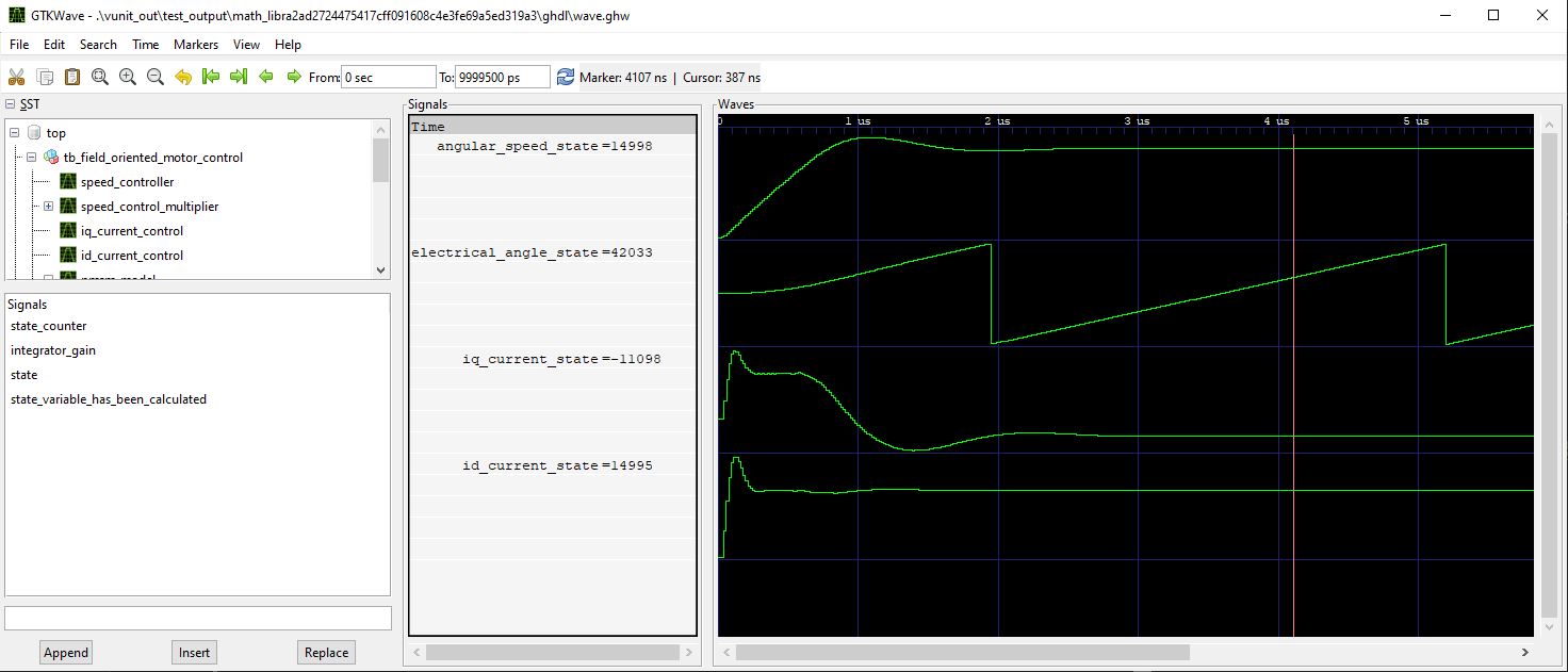
The project is compiled to cyclone 10 lp FPGA and the speed and $i_q(t)$ current are captured using UART. The speed reference is stepped between 20 000 and -10 000 and the load torque is stepped in the opposite direction at both speeds. The load step is seen as the transient in the middle of the speed curve.

The corresponding $i_q(t)$ has a current step at the speed reference change. This is because the simulation model has quite high friction torque that increases with the speed. The speed controller has maximum current reference limit at +/-32 000 which can be seen as the current is not increased past those points during a load step.

Calculation delay and resource use

The resourse usage is shown in Figure 5. The total number of 18×18 multipliers is 6, with both the model and the controller using 3 multipliers. The motor simulator is in the motor_control_hardware layer and the feedback control algorithm is implemented in the motor_control_data_processing layer. The motor model requires less than 1000 logic units and 3 multipliers and the control algorithm requires approximately the same amount.

The motor control calculations run in 17 clock cycles from start to finish. Since the FPGA is clocked at 120Mhz this means that the feedback calculation has a ~150ns calculation delay. This is with all controls running with their own multipliers and multiplier having 3 pipeline delays.

Coordinate transforms

In a real system we would get the motor currents as 3 phase currents measured from the three motor cables instead of the dq quantities used here. In order to measure dq currents we need to transform them from the three phase abc currents. The transforms that are used for this are called Clarke (31)-(32) and Park (33)-(34) transforms. To transform the 3-phase currenst to d and q oriented counterparts we use first transform (31) to $i_a(t), i_b(t)$ and $i_c(t)$ which gives $i_\alpha(t)$ and $i_\beta(t)$ . These are then transformed into $i_d(t)$ and $i_q(t)$ with (33). After the feedback calculation has produced the control voltages $v_d(t)$ and $v_q(t)$ we use (34) and in some case also (33) to produce the voltages for the inverters modulator which then produces gate signals for the semiconductors that actually drive the motor.

\begin{align} \begin{bmatrix} \alpha \\ \beta \end{bmatrix} &= \frac{2}{3} \begin{bmatrix} \phantom{-}1 & -\frac{1}{2} & -\frac{1}{2} \\[0.5em] \phantom{-}0 & \phantom{-}\frac{\sqrt{2}}{3} & -\frac{\sqrt{2}}{3} \end{bmatrix} \begin{bmatrix} a \\ b \\ c \end{bmatrix} \\[3em] \begin{bmatrix} a \\ b \\ c \end{bmatrix} &= \frac{3}{2} \begin{bmatrix} \phantom{-}1 & \phantom{-}0 \\[0.5em] -\frac{1}{2} & \phantom{-}\frac{\sqrt{3}}{2}\\[0.5em] -\frac{1}{2} & -\frac{1}{2} \end{bmatrix} \begin{bmatrix} \alpha \\ \beta \end{bmatrix} \end{align}

\begin{align} \begin{bmatrix} d\\ q \\ \end{bmatrix} &= \begin{bmatrix} cos(\phi_e) & -sin(\phi_e) \\[0.5em] sin(\phi_e) & \phantom{-}cos(\phi_e) \end{bmatrix} \begin{bmatrix} \alpha \\ \beta \end{bmatrix} \\[2em] \begin{bmatrix} \alpha \\ \beta \end{bmatrix} &= \begin{bmatrix} \phantom{-}cos(\phi_e) & sin(\phi_e) \\[0.5em] -sin(\phi_e) & cos(\phi_e) \end{bmatrix} \begin{bmatrix} d\\ q \end{bmatrix} \end{align}

All of the complexity of the coordinate transforms is in the estimation of the angle $\phi_e$ in (33) and (34) as the transforms themselves can be used as is with no further tricks. The angle can either be measured with a sensor, or calculated from a model of the electrical part of the motor, which is referred to as observer in the control literature.

Notes on the motor control simulation project

The project here is only the bare minimum that is able to simulate a motor and a controller for it as it is missing some basic features. The system architecture already has a module for the system level controls that would allow for starting and stopping the control. The system control would also include the tripping by stopping the control if excess current was measured.

The motor simulator also transmits the currents in dq quantities. In order to better simulate a real motor drive, the current should be transformed into 3 phase quantities. The electrical angle of the motor is also not available in a real system. So to improve the simulation an angle estimation block with either model for either the measurement device or observer could be added.

The motor control project architecture is more deeply covered in next post. Although the project is tested with Intel Cyclone 10 lp fpga, the code is designed to be compiled to any other FPGA. Especially the separation of the tool and FPGA specific design units reduces the need of redesign as the application code is shared and the specific modules are designed to create the same interface.

Field Oriented motor control with VHDL

Modeling and control of a Permanent Magnet Electric Motor

Motor mechanical model

Torque in electrical motors

Lorenz torque

Reluctance torque

Motor mechanical model

Motor electrical model

Field Oriented Current Control

Speed control

VHDL implementation of motor model and control

Mechanical model

Electrical model

Motor current control

Motor Speed control

Test with FPGA

FPGA simulation

Calculation delay and resource use

Coordinate transforms

Notes on the motor control simulation project

1 thought on “Field Oriented motor control with VHDL”

Leave a Comment Cancel Reply

About Hardware Descriptions